In one of the previous labs, we’ve already uploaded three CSV files that we need for this lab.
To ensure that you have all the necessary data, open the LH_Fabric_Bootcamp lakehouse, expand the Files area, and select the orders folder. You should see three CSV files, as displayed below:
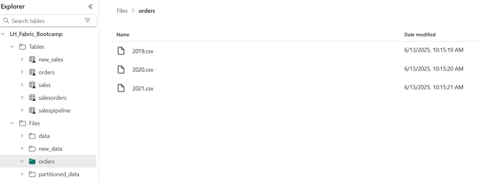
In medallion architecture, this is considered a bronze layer, since we are storing the data in its raw form. Therefore, the orders folder in the Files area of the lakehouse is considered a bronze layer for our lab.
Transform data and load to silver layer Delta table
Now that you have some data in the bronze layer of the lakehouse, you can use a notebook to transform the data and load it into a delta table in the silver layer.
- On the Home page while viewing the contents of the orders folder in your data lake, in the Open notebook menu in the top ribbon, select New notebook.
After a few seconds, a new notebook containing a single cell will open. Notebooks are made up of one or more cells that can contain code or markdown (formatted text).
- When the notebook opens, rename it to Transform data for Silver by selecting the Notebook 1 text at the top left of the notebook and entering the new name.
- Select the existing cell in the notebook, that contains some sample code. Highlight and delete these two lines and paste the following code into the cell:
from pyspark.sql.types import *

# Create the schema for the table
orderSchema = StructType([
    StructField("SalesOrderNumber", StringType()),
    StructField("SalesOrderLineNumber", IntegerType()),
    StructField("OrderDate", DateType()),
    StructField("CustomerName", StringType()),
    StructField("Email", StringType()),
    StructField("Item", StringType()),
    StructField("Quantity", IntegerType()),
    StructField("UnitPrice", FloatType()),
    StructField("Tax", FloatType())
    ])

# Import all files from bronze folder of lakehouse
df = spark.read.format("csv").option("header", "true").schema(orderSchema).load("Files/orders/*.csv")

# Display the first 10 rows of the dataframe to preview your data
display(df.head(10))
- Use the **▷ (Run cell)** button on the left of the cell to run the code.
- When the cell command has completed, review the output below the cell, which should look similar to this:
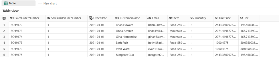
The code you ran loaded the data from the CSV files in the orders folder into a Spark dataframe, and then displayed the first few rows of the dataframe.
- Now you’ll add columns for data validation and cleanup, using a PySpark dataframe to add columns and update the values of some of the existing columns. Use the + Code button to add a new code block and add the following code to the cell:
from pyspark.sql.functions import when, lit, col, current_timestamp, input_file_name

# Add columns IsFlagged, CreatedTS and ModifiedTS
df = df.withColumn("FileName", input_file_name()) \
    .withColumn("IsFlagged", when(col("OrderDate") < '2019-08-01',True).otherwise(False)) \
    .withColumn("CreatedTS", current_timestamp()).withColumn("ModifiedTS", current_timestamp())

# Update CustomerName to "Unknown" if CustomerName null or empty
df = df.withColumn("CustomerName", when((col("CustomerName").isNull() | (col("CustomerName")=="")),lit("Unknown")).otherwise(col("CustomerName")))
The first line of the code imports the necessary functions from PySpark. You’re then adding new columns to the dataframe so you can track the source file name, whether the order was flagged as being before the fiscal year of interest, and when the row was created and modified.
Finally, you’re updating the CustomerName column to “Unknown” if it’s null or empty.
- Run the cell to execute the code using the **▷ (Run cell)** button.
- Next, you’ll define the schema for the sales_silver table in the sales database using Delta Lake format. Create a new code block and add the following code to the cell:
# Define the schema for the sales_silver table

from pyspark.sql.types import *
from delta.tables import *

DeltaTable.createIfNotExists(spark) \
    .tableName("sales_silver") \
    .addColumn("SalesOrderNumber", StringType()) \
    .addColumn("SalesOrderLineNumber", IntegerType()) \
    .addColumn("OrderDate", DateType()) \
    .addColumn("CustomerName", StringType()) \
    .addColumn("Email", StringType()) \
    .addColumn("Item", StringType()) \
    .addColumn("Quantity", IntegerType()) \
    .addColumn("UnitPrice", FloatType()) \
    .addColumn("Tax", FloatType()) \
    .addColumn("FileName", StringType()) \
    .addColumn("IsFlagged", BooleanType()) \
    .addColumn("CreatedTS", DateType()) \
    .addColumn("ModifiedTS", DateType()) \
    .execute()
- Run the cell to execute the code using the **▷ (Run cell)** button.
- Select the … in the Tables section of the Explorer pane and select Refresh. You should now see the new sales_silver table listed. The ▲ (triangle icon) indicates that it’s a Delta table.
- Now you’re going to perform an upsert operation on a Delta table, updating existing records based on specific conditions and inserting new records when no match is found. Add a new code block and paste the following code:
# Update existing records and insert new ones based on a condition defined by the columns SalesOrderNumber, OrderDate, CustomerName, and Item.

from delta.tables import *

deltaTable = DeltaTable.forPath(spark, 'Tables/sales_silver')

dfUpdates = df

deltaTable.alias('silver') \
  .merge(
    dfUpdates.alias('updates'),
    'silver.SalesOrderNumber = updates.SalesOrderNumber and silver.OrderDate = updates.OrderDate and silver.CustomerName = updates.CustomerName and silver.Item = updates.Item'
  ) \
   .whenMatchedUpdate(set =
    {

    }
  ) \
 .whenNotMatchedInsert(values =
    {
      "SalesOrderNumber": "updates.SalesOrderNumber",
      "SalesOrderLineNumber": "updates.SalesOrderLineNumber",
      "OrderDate": "updates.OrderDate",
      "CustomerName": "updates.CustomerName",
      "Email": "updates.Email",
      "Item": "updates.Item",
      "Quantity": "updates.Quantity",
      "UnitPrice": "updates.UnitPrice",
      "Tax": "updates.Tax",
      "FileName": "updates.FileName",
      "IsFlagged": "updates.IsFlagged",
      "CreatedTS": "updates.CreatedTS",
      "ModifiedTS": "updates.ModifiedTS"
    }
  ) \
    .execute()
- Run the cell to execute the code using the **▷ (Run cell)** button.
This operation is important because it enables you to update existing records in the table based on the values of specific columns, and insert new records when no match is found. This is a common requirement when you’re loading data from a source system that may contain updates to existing and new records.
You now have data in your silver delta table that is ready for further transformation and modeling.
Explore data in the silver layer using the SQL endpoint
Now that you have data in your silver layer, you can use the SQL analytics endpoint to explore the data and perform some basic analysis. This is useful if you’re familiar with SQL and want to do some basic exploration of your data. In this exercise, we’re using the SQL endpoint view in Fabric, but you can use other tools like SQL Server Management Studio (SSMS).
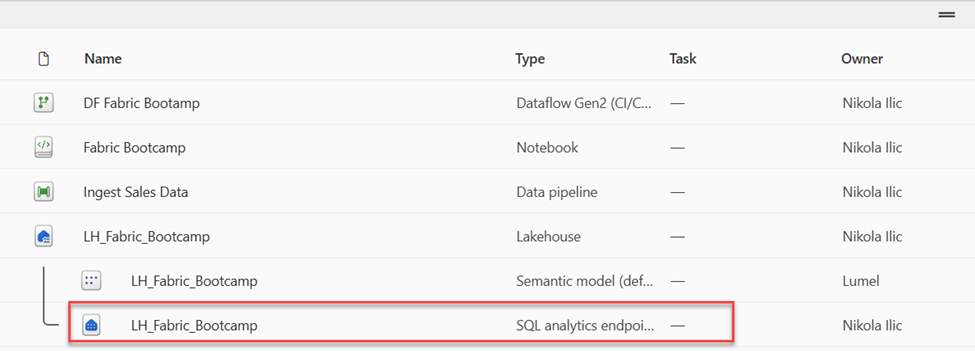
- Navigate back to your workspace and notice that you now have several items listed. Select the Sales SQL analytics endpoint to open your lakehouse in the SQL analytics endpoint view.
- Select New SQL query from the ribbon, which will open a SQL query editor. Note that you can rename your query using the … menu item next to the existing query name in the Explorer pane.
Next, you’ll run two sql queries to explore the data.
- Paste the following query into the query editor and select Run:
SELECT YEAR(OrderDate) AS Year
    , CAST (SUM(Quantity * (UnitPrice + Tax)) AS DECIMAL(12, 2)) AS TotalSales
FROM sales_silver
GROUP BY YEAR(OrderDate)
ORDER BY YEAR(OrderDate)
This query calculates the total sales for each year in the sales_silver table.
- Next, you’ll review which customers are purchasing the most (in terms of quantity). Paste the following query into the query editor and select Run:
SELECT TOP 10 CustomerName, SUM(Quantity) AS TotalQuantity
FROM sales_silver
GROUP BY CustomerName
ORDER BY TotalQuantity DESC
This query calculates the total quantity of items purchased by each customer in the sales_silver table, and then returns the top 10 customers in terms of quantity.
Data exploration in the silver layer is useful for basic analysis, but you’ll need to transform the data further and model it into a star schema to enable more advanced analysis and reporting. We’ll do that in the next section.
Transform data for gold layer
You have successfully taken data from your bronze layer, transformed it, and loaded it into a silver Delta table. Now you’ll use a new notebook to transform the data further, model it into a star schema, and load it into gold Delta tables.
You could have done all of this in a single notebook, but for this exercise, we’re using separate notebooks to demonstrate the process of transforming data from bronze to silver and then from silver to gold. This can help with debugging, troubleshooting, and reuse.
- Return to the workspace home page and create a new notebook called Transform data for Gold.
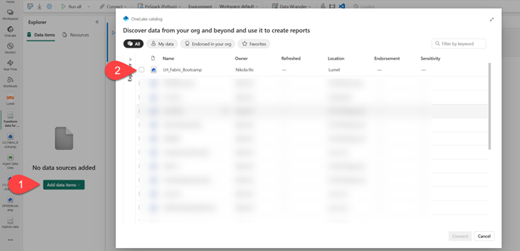
- In the Explorer pane, add your LH_Fabric_Bootcamp lakehouse by selecting Add data items and then selecting the LH_Fabric_Bootcamp lakehouse. You should see the sales_silver table listed in the Tables section of the explorer pane.
- In the existing code block, remove the commented text and add the following code to load data to your dataframe and start building your star schema, then run it:
# Load data to the dataframe as a starting point to create the gold layer
df = spark.read.table("sales_silver")
- Add a new code block and paste the following code to create your date dimension table and run it:
from pyspark.sql.types import *
from delta.tables import*

# Define the schema for the dimdate_gold table
DeltaTable.createIfNotExists(spark) \
    .tableName("dimdate_gold") \
    .addColumn("OrderDate", DateType()) \
    .addColumn("Day", IntegerType()) \
    .addColumn("Month", IntegerType()) \
    .addColumn("Year", IntegerType()) \
    .addColumn("mmmyyyy", StringType()) \
    .addColumn("yyyymm", StringType()) \
    .execute()
Tip: You can run the display(df) command at any time to check the progress of your work. In this case, you’d run ‘display(dfdimDate_gold)’ to see the contents of the dimDate_gold dataframe.
- In a new code block, add and run the following code to create a dataframe for your date dimension, dimdate_gold:
from pyspark.sql.functions import col, dayofmonth, month, year, date_format

# Create dataframe for dimDate_gold

dfdimDate_gold = df.dropDuplicates(["OrderDate"]).select(col("OrderDate"), \
        dayofmonth("OrderDate").alias("Day"), \
        month("OrderDate").alias("Month"), \
        year("OrderDate").alias("Year"), \
        date_format(col("OrderDate"), "MMM-yyyy").alias("mmmyyyy"), \
        date_format(col("OrderDate"), "yyyyMM").alias("yyyymm"), \
    ).orderBy("OrderDate")

# Display the first 10 rows of the dataframe to preview your data

display(dfdimDate_gold.head(10))
You’re separating the code out into new code blocks so that you can understand and watch what’s happening in the notebook as you transform the data.
- In another new code block, add and run the following code to update the date dimension as new data comes in:
from delta.tables import *

deltaTable = DeltaTable.forPath(spark, 'Tables/dimdate_gold')

dfUpdates = dfdimDate_gold

deltaTable.alias('gold') \
  .merge(
    dfUpdates.alias('updates'),
    'gold.OrderDate = updates.OrderDate'
  ) \
   .whenMatchedUpdate(set =
    {

    }
  ) \
 .whenNotMatchedInsert(values =
    {
      "OrderDate": "updates.OrderDate",
      "Day": "updates.Day",
      "Month": "updates.Month",
      "Year": "updates.Year",
      "mmmyyyy": "updates.mmmyyyy",
      "yyyymm": "updates.yyyymm"
    }
  ) \
.execute()
The date dimension is now set up. Now you’ll create your customer dimension.
- To build out the customer dimension table, add a new code block, paste and run the following code:
from pyspark.sql.types import *
from delta.tables import *

# Create customer_gold dimension delta table
DeltaTable.createIfNotExists(spark) \
    .tableName("dimcustomer_gold") \
    .addColumn("CustomerName", StringType()) \
    .addColumn("Email",  StringType()) \
    .addColumn("First", StringType()) \
    .addColumn("Last", StringType()) \
    .addColumn("CustomerID", LongType()) \
    .execute()
- In a new code block, add and run the following code to drop duplicate customers, select specific columns, and split the “CustomerName” column to create “First” and “Last” name columns:
from pyspark.sql.functions import col, split

# Create customer_silver dataframe

dfdimCustomer_silver = df.dropDuplicates(["CustomerName","Email"]).select(col("CustomerName"),col("Email")) \
    .withColumn("First",split(col("CustomerName"), " ").getItem(0)) \
    .withColumn("Last",split(col("CustomerName"), " ").getItem(1))

# Display the first 10 rows of the dataframe to preview your data

display(dfdimCustomer_silver.head(10))
Here, you have created a new dataframe dfdimCustomer_silver, by performing various transformations such as dropping duplicates, selecting specific columns, and splitting the “CustomerName” column to create “First” and “Last” name columns. The result is a dataframe with cleaned and structured customer data, including separate “First” and “Last” name columns extracted from the “CustomerName” column.
- Next we’ll create the ID column for our customers. In a new code block, paste and run the following:
from pyspark.sql.functions import monotonically_increasing_id, col, when, coalesce, max, lit

dfdimCustomer_temp = spark.read.table("dimCustomer_gold")

MAXCustomerID = dfdimCustomer_temp.select(coalesce(max(col("CustomerID")),lit(0)).alias("MAXCustomerID")).first()[0]

dfdimCustomer_gold = dfdimCustomer_silver.join(dfdimCustomer_temp,(dfdimCustomer_silver.CustomerName == dfdimCustomer_temp.CustomerName) & (dfdimCustomer_silver.Email == dfdimCustomer_temp.Email), "left_anti")

dfdimCustomer_gold = dfdimCustomer_gold.withColumn("CustomerID",monotonically_increasing_id() + MAXCustomerID + 1)

# Display the first 10 rows of the dataframe to preview your data
display(dfdimCustomer_gold.head(10))
Here you’re cleaning and transforming customer data (dfdimCustomer_silver) by performing a left anti join to exclude duplicates that already exist in the dimCustomer_gold table, and then generating unique CustomerID values using the monotonically_increasing_id() function.
- Now you’ll ensure that your customer table remains up-to-date as new data comes in. In a new code block, paste and run the following:
from delta.tables import *

deltaTable = DeltaTable.forPath(spark, 'Tables/dimcustomer_gold')

dfUpdates = dfdimCustomer_gold

deltaTable.alias('gold') \
  .merge(
    dfUpdates.alias('updates'),
    'gold.CustomerName = updates.CustomerName AND gold.Email = updates.Email'
  ) \
   .whenMatchedUpdate(set =
    {

    }
  ) \
 .whenNotMatchedInsert(values =
    {
      "CustomerName": "updates.CustomerName",
      "Email": "updates.Email",
      "First": "updates.First",
      "Last": "updates.Last",
      "CustomerID": "updates.CustomerID"
    }
  ) \
.execute()
- Now you’ll repeat those steps to create your product dimension. In a new code block, paste and run the following:
from pyspark.sql.types import *
from delta.tables import *

DeltaTable.createIfNotExists(spark) \
    .tableName("dimproduct_gold") \
    .addColumn("ItemName", StringType()) \
    .addColumn("ItemID", LongType()) \
    .addColumn("ItemInfo", StringType()) \
    .execute()
- Add another code block to create the product_silver dataframe.
from pyspark.sql.functions import col, split, lit, when

# Create product_silver dataframe

dfdimProduct_silver = df.dropDuplicates(["Item"]).select(col("Item")) \
    .withColumn("ItemName",split(col("Item"), ", ").getItem(0)) \
    .withColumn("ItemInfo",when((split(col("Item"), ", ").getItem(1).isNull() | (split(col("Item"), ", ").getItem(1)=="")),lit("")).otherwise(split(col("Item"), ", ").getItem(1)))

# Display the first 10 rows of the dataframe to preview your data
display(dfdimProduct_silver.head(10))
- Now you’ll create IDs for your dimProduct_gold table. Add the following syntax to a new code block and run it:
from pyspark.sql.functions import monotonically_increasing_id, col, lit, max, coalesce

#dfdimProduct_temp = dfdimProduct_silver
dfdimProduct_temp = spark.read.table("dimProduct_gold")

MAXProductID = dfdimProduct_temp.select(coalesce(max(col("ItemID")),lit(0)).alias("MAXItemID")).first()[0]

dfdimProduct_gold = dfdimProduct_silver.join(dfdimProduct_temp,(dfdimProduct_silver.ItemName == dfdimProduct_temp.ItemName) & (dfdimProduct_silver.ItemInfo == dfdimProduct_temp.ItemInfo), "left_anti")

dfdimProduct_gold = dfdimProduct_gold.withColumn("ItemID",monotonically_increasing_id() + MAXProductID + 1)

# Display the first 10 rows of the dataframe to preview your data
display(dfdimProduct_gold.head(10))
This calculates the next available product ID based on the current data in the table, assigns these new IDs to the products, and then displays the updated product information.
- Similar to what you’ve done with your other dimensions, you need to ensure that your product table remains up-to-date as new data comes in. In a new code block, paste and run the following:
from delta.tables import *

deltaTable = DeltaTable.forPath(spark, 'Tables/dimproduct_gold')

dfUpdates = dfdimProduct_gold

deltaTable.alias('gold') \
  .merge(
        dfUpdates.alias('updates'),
        'gold.ItemName = updates.ItemName AND gold.ItemInfo = updates.ItemInfo'
        ) \
        .whenMatchedUpdate(set =
        {

        }
        ) \
        .whenNotMatchedInsert(values =
         {
          "ItemName": "updates.ItemName",
          "ItemInfo": "updates.ItemInfo",
          "ItemID": "updates.ItemID"
          }
          ) \
        .execute()
Now that you have your dimensions built out, the final step is to create the fact table.
- In a new code block, paste and run the following code to create the fact table:
from pyspark.sql.types import *
from delta.tables import *

DeltaTable.createIfNotExists(spark) \
    .tableName("factsales_gold") \
    .addColumn("CustomerID", LongType()) \
    .addColumn("ItemID", LongType()) \
    .addColumn("OrderDate", DateType()) \
    .addColumn("Quantity", IntegerType()) \
    .addColumn("UnitPrice", FloatType()) \
    .addColumn("Tax", FloatType()) \
    .execute()
- In a new code block, paste and run the following code to create a new dataframe to combine sales data with customer and product information include customer ID, item ID, order date, quantity, unit price, and tax:
from pyspark.sql.functions import col

dfdimCustomer_temp = spark.read.table("dimCustomer_gold")
dfdimProduct_temp = spark.read.table("dimProduct_gold")

df = df.withColumn("ItemName",split(col("Item"), ", ").getItem(0)) \
    .withColumn("ItemInfo",when((split(col("Item"), ", ").getItem(1).isNull() | (split(col("Item"), ", ").getItem(1)=="")),lit("")).otherwise(split(col("Item"), ", ").getItem(1))) \


# Create Sales_gold dataframe

dffactSales_gold = df.alias("df1").join(dfdimCustomer_temp.alias("df2"),(df.CustomerName == dfdimCustomer_temp.CustomerName) & (df.Email == dfdimCustomer_temp.Email), "left") \
        .join(dfdimProduct_temp.alias("df3"),(df.ItemName == dfdimProduct_temp.ItemName) & (df.ItemInfo == dfdimProduct_temp.ItemInfo), "left") \
    .select(col("df2.CustomerID") \
        , col("df3.ItemID") \
        , col("df1.OrderDate") \
        , col("df1.Quantity") \
        , col("df1.UnitPrice") \
        , col("df1.Tax") \
    ).orderBy(col("df1.OrderDate"), col("df2.CustomerID"), col("df3.ItemID"))
# Display the first 10 rows of the dataframe to preview your data
display(dffactSales_gold.head(10))
- Now you’ll ensure that sales data remains up-to-date by running the following code in a new code block:
from delta.tables import *

deltaTable = DeltaTable.forPath(spark, 'Tables/factsales_gold')

dfUpdates = dffactSales_gold

deltaTable.alias('gold') \
  .merge(
    dfUpdates.alias('updates'),
    'gold.OrderDate = updates.OrderDate AND gold.CustomerID = updates.CustomerID AND gold.ItemID = updates.ItemID'
  ) \
   .whenMatchedUpdate(set =
    {

    }
  ) \
 .whenNotMatchedInsert(values =
    {
      "CustomerID": "updates.CustomerID",
      "ItemID": "updates.ItemID",
      "OrderDate": "updates.OrderDate",
      "Quantity": "updates.Quantity",
      "UnitPrice": "updates.UnitPrice",
      "Tax": "updates.Tax"
    }
  ) \
.execute()
Here you’re using Delta Lake’s merge operation to synchronize and update the factsales_gold table with new sales data (dffactSales_gold). The operation compares the order date, customer ID, and item ID between the existing data (silver table) and the new data (updates dataframe), updating matching records and inserting new records as needed.
Wow, what a lab it was! You completed so many tasks, and you should be proud of yourself! You now have a curated, efficient gold layer that can be used for reporting and analysis.
And, that’s a wrap! You’ve completed all the labs, and you should now be well equipped to start building scalable and robust analytics solutions using Microsoft Fabric. Well done!